Show code
library(pacman)
p_load(magrittr, tidyverse, psych, dplyr, ggplot2, haven, janitor, readxl, writexl, knitr, kableExtra, scales, tibble, tidyr, labelled, survey)![]()
library(pacman)
p_load(magrittr, tidyverse, psych, dplyr, ggplot2, haven, janitor, readxl, writexl, knitr, kableExtra, scales, tibble, tidyr, labelled, survey)This project examines bone health in adults using survey data from the NHANES data library, with a focus on identifying individuals at an elevated risk of osteoporosis. Current screening criteria consider only gender and age and are therefore limited. Bone mineral density measurements and common risk indicators were used to characterize patterns of risk across age and gender groups. The analysis also explores how current age-based screening recommendations may miss individuals with meaningful bone-health risk.
The findings aim to support earlier identification of high-risk populations and inform more targeted approaches to bone-health assessment.
This analysis used publicly available data from the 2005–2006 National Health and Nutrition Examination Survey (NHANES). Demographic, body measurement, dual-energy X-ray absorptiometry (DXA) bone density, osteoporosis history, smoking, and physical activity datasets were merged at the individual level using the NHANES respondent identifier. Bone-health risk was defined using lumbar spine DXA measures and established clinical thresholds, supplemented by well-recognized behavioral and clinical risk factors. All analyses were descriptive and exploratory, intended to characterize screening gaps rather than to support clinical diagnosis.
Multiple NHANES data sets were integrated in this analysis, including demographic information, body measurements, DXA bone density measurements, osteoporosis and fracture history, smoking behavior, and physical activity data. Together, these data sets provide a comprehensive view of bone health, relevant risk factors, and population-level screening patterns across adults.
# Data was read in, it was a .xpt file
# Data files are kept in a folder within the project folder called "data" - if replicating do the same for this chunk to run
bio <- read_xpt("data/DEMO_D.xpt")

bmx <- read_xpt("data/BMX_D.xpt")

dxa <- read_xpt("data/dxx_d.xpt")

osteo <- read_xpt("data/OSQ_D.xpt")

smoke <- read_xpt("data/SMQ_D.xpt")

activity <- read_xpt("data/PAQ_D.xpt")The NHANES DXA data include multiple imputed records per participant (due to missing data). While formal epidemiologic analyses would typically run analyses on all imputations, this analytics exercise used a single imputation (MULT = 1). Furthermore, observations were excluded if they did not complete a full and valid exam (DXAEXSTS = 1).
# Selecting single imputation and removing incomplete exam data
dxa_clean <- dxa %>%
  dplyr::filter(`_MULT_` == 1) %>%
dplyr::filter(DXAEXSTS == 1)Relevant variables were selected from each NHANES data set to support the assessment of bone health, fracture risk, and screening eligibility. Demographic variables were used to characterize the study population and define age- and gender-based screening criteria. Body measurement variables provided objective indicators of body mass, which is a known risk factor for low bone density. DXA-derived bone mineral density measures were used to characterize skeletal health, with lumbar spine density serving as the primary site for bone-risk classification. Osteoporosis, smoking, and physical activity variables were included to capture established clinical and lifestyle risk factors associated with fracture risk.
All variables were selected based on their clinical relevance, availability in the NHANES 2005–2006 cycle, and suitability for population-level risk stratification rather than individual diagnosis.
Several derived variables were created from the selected NHANES variables to support bone-health risk stratification.
Low body mass index (low_bmi) was defined as a body mass index (BMI) below 18.5 kg/m². This threshold reflects underweight status and is a well-established risk factor for reduced bone density and increased fracture risk.
Lumbar spine T-score (tscore_spine) was calculated by standardizing lumbar spine BMD using published reference values for young healthy adults (Xue et al., 2021). The resulting T-score represents the number of standard deviations an individual’s bone density differs from the reference mean and allows alignment with widely used clinical conventions. Based on this T-score, spine_class was defined to indicate normal bone density, osteopenia, or osteoporosis using conventional cut-points (≥ −1.0, −1.0 to −2.5, and ≤ −2.5, respectively). These classifications are used for contextual interpretation and not for clinical diagnosis.
Prior fracture history (prior_fracture) was defined as a history of self-reported fracture at the hip, wrist, or spine. Individuals reporting a fracture at any of these sites were flagged as having a prior fracture, which is a strong indicator of future fracture risk.
Smoking status (smoker_status) was derived using a combination of lifetime smoking history and current smoking behavior. Individuals who reported never having smoked at least 100 cigarettes in their lifetime were classified as never smokers. Those who had smoked at least 100 cigarettes and reported currently smoking every day or on some days were classified as current smokers. Individuals who had smoked at least 100 cigarettes but reported not currently smoking were classified as former smokers. This categorization reflects cumulative smoking exposure relevant to bone health rather than short-term smoking behavior.
Low physical activity (low_activity) was defined as reporting neither moderate nor vigorous physical activity during the past 30 days. Low levels of physical activity are associated with reduced mechanical loading of bone and increased fracture risk, particularly in older adults.
Together, these derived variables provide clinically meaningful and interpretable indicators of bone-health risk that support population-level cohort definition and analysis without implying individual-level diagnosis.
# Variable selection

# Bio
bio_sel <- bio %>%
  dplyr::select(
    SEQN,         # ID
    RIDAGEYR,     # age (years)
    RIAGENDR,     # gender (1 = male, 2 = female)
    RIDRETH1,     # race
    WTMEC2YR,     # statistical exam weight
    SDMVPSU,      # Masked Variance Pseudo-PSU
    SDMVSTRA      # Masked Variance Pseudo-Stratum
  )


# bmx
bmx_sel <- bmx %>%
  dplyr::select(
    SEQN,         # ID
    BMXBMI        # BMI
  ) %>%
  mutate(
    low_bmi = if_else(BMXBMI < 18.5, 1, 0)
  )

# dxa

# Reference values for T-scores
ref_spine_mean   <- 1.065
ref_spine_sd     <- 0.122

dxa_sel <- dxa_clean %>%
  dplyr::select(
    SEQN,         # ID
    DXXLSBMD,     # Lumbar Spine BMD (g/cm^2)
  ) %>%
    mutate(
    # Calculate T-scores
    tscore_spine   = (DXXLSBMD   - ref_spine_mean)   / ref_spine_sd,

    spine_class = case_when(
      tscore_spine >= -1.0 ~ 0,                       # 0 = normal
      tscore_spine < -1.0 & tscore_spine > -2.5 ~ 1,  # 1 = osteopenia
      tscore_spine <= -2.5 ~ 2,                       # 2 = osteoporosis
      TRUE ~ NA_real_
    )
  )


# osteo
osteo_sel <- osteo %>%
  dplyr::select(
    SEQN,     # ID
    OSQ010A,  # broken/fractured hip (yes = 1, no = 2)
    OSQ010B,  # broken/fractured wrist
    OSQ010C,  # broken/fractured spine
    OSQ060   # "Ever told had osteoporosis/brittle bones"
  ) %>%
  mutate(
    prior_fracture = if_else(OSQ010A == 1 | OSQ010B == 1 | OSQ010C == 1, 1, 0)
  )

# smoke
smoke_sel <- smoke %>%
  dplyr::select(
    SEQN,       # ID
    SMQ020,     # smoked at least 100 cigarettes in life (yes = 1, no = 2)
    SMD030,     # Age started smoking cigarettes regularly
    SMQ040,     # Do you now smoke cigarettes (1 = everyday, 2 = some days, 3 = not at all)
  ) %>%
  mutate(
    smoker_status = case_when(
      SMQ020 == 2 ~ 0,                          # Never smoker
      SMQ020 == 1 & SMQ040 %in% c(1, 2) ~ 1,    # Current smoker
      SMQ020 == 1 & SMQ040 == 3 ~ 2,            # Former smoker
      TRUE ~ NA_real_                           # Missing/other
    )
  )

# activity
activity_sel <- activity %>%
  dplyr::select(
    SEQN,       # ID
    PAD200,     # Vigorous activity over past 30 days (1 = yes, 2 = no, 3 = unable)
    PAD320,     # Moderate activity over past 30 days (1 = yes, 2 = no, 3 = unable)
  ) %>%
  mutate(
    low_activity = if_else(
      PAD200 == 2 & PAD320 == 2,  # no vigorous AND no moderate activity
      1, 0
    )
)The selected NHANES data sets were merged into a single analytic data set to enable integrated analysis across bone density measurements, demographic characteristics, and relevant risk factors. All data sets were linked using the NHANES respondent sequence number, which uniquely identifies each participant across survey components. Bone density data served as the anchor for the merged data set, ensuring that all included individuals had valid DXA measurements. Additional data from demographic, body measurement, osteoporosis, smoking, and physical activity components were joined to enrich the analytic data set with clinically relevant context while preserving one record per participant.
# Merging of data sets

data <- bio_sel %>%
  inner_join(dxa_sel,  by = "SEQN") %>%
  left_join(bmx_sel,   by = "SEQN") %>%
  left_join(osteo_sel, by = "SEQN") %>%
  left_join(smoke_sel, by = "SEQN") %>%
left_join(activity_sel, by = "SEQN") The analysis was restricted to adults aged 20 years and older. Several risk proxy variables (e.g., smoking history and fracture history) are not collected for children and adolescents in NHANES. Restricting the analytic sample to adults ensures consistent measurement of all indicators and avoids misclassification due to age-based survey skip patterns.
# Filtering out children and mutating NA for low BMI to 0
data %<>%
dplyr::filter(RIDAGEYR >= 20)The data set was examined for overall missingness to quantify the extent of incomplete records and to assess whether missing data posed a material risk to analytic validity. A meaningful amount of missing data was detected so variable-level analysis was conducted.
# Overall missingness summary
na_summary <- data %>%
  summarise(
    total_cells = n() * ncol(data),
    total_missing = sum(is.na(.)),
    pct_missing = round(100 * total_missing / total_cells, 2)
  )

kable(na_summary,
      col.names = c("Total Cells", "Total Cells Missing", "% Missing"),
      align = c("l", "l", "l"),
caption = "Overall Missing Cells Summary")| Total Cells | Total Cells Missing | % Missing |
|---|---|---|
| 74568 | 3264 | 4.38 |
Missingness was then evaluated at the variable level to identify systematic patterns or structural gaps, allowing informed decisions about exclusion or conservative handling of incomplete fields.
# Variable-level missingness
na_check <- data %>%
  summarise(across(
    everything(),
    ~ sum(is.na(.)),
    .names = "na_{.col}"
  )) %>%
  pivot_longer(
    everything(),
    names_to = "variable",
    values_to = "missing_n"
  ) %>%
  mutate(
    variable = gsub("^na_", "", variable),
    pct_missing = round(100 * missing_n / nrow(data), 2)
  ) %>%
  arrange(desc(missing_n))

kable(na_check,
      col.names = c("Variable", "Missing Count", "% Missing"),
      align = c("l", "l", "l"),
caption = "Variable-level Missing Cells Summary")| Variable | Missing Count | % Missing |
|---|---|---|
| SMD030 | 1619 | 52.11 |
| SMQ040 | 1619 | 52.11 |
| BMXBMI | 12 | 0.39 |
| low_bmi | 12 | 0.39 |
| smoker_status | 2 | 0.06 |
| SEQN | 0 | 0.00 |
| RIDAGEYR | 0 | 0.00 |
| RIAGENDR | 0 | 0.00 |
| RIDRETH1 | 0 | 0.00 |
| WTMEC2YR | 0 | 0.00 |
| SDMVPSU | 0 | 0.00 |
| SDMVSTRA | 0 | 0.00 |
| DXXLSBMD | 0 | 0.00 |
| tscore_spine | 0 | 0.00 |
| spine_class | 0 | 0.00 |
| OSQ010A | 0 | 0.00 |
| OSQ010B | 0 | 0.00 |
| OSQ010C | 0 | 0.00 |
| OSQ060 | 0 | 0.00 |
| prior_fracture | 0 | 0.00 |
| SMQ020 | 0 | 0.00 |
| PAD200 | 0 | 0.00 |
| PAD320 | 0 | 0.00 |
| low_activity | 0 | 0.00 |
The missingness in the smoking-related variables (SMD030 & SMD030) was not problematic as they are automatically coded as NA if the individual has NOT smoked more than 100 cigarettes in their lifetime making them a non-smoker in the smoker_status variable.
A small number of observations (n = 12) had missing body mass index values. These cases were retained in the analysis, with the low-BMI risk proxy conservatively defaulted to absent to avoid inflating risk estimates.
The two individuals who selected “Don’t know” in relation to their smoking habits have been retained and smoking status conservatively defaulted to absent to avoid inflating risk estimates.
# Mutating NA for low BMI to 0 and NA smoking status to 0
data %<>%
  mutate(
    low_bmi = if_else(is.na(low_bmi), 0, low_bmi),
    smoker_status = if_else(is.na(smoker_status), 0, smoker_status)
)Three cohorts were defined to support evaluation of bone-health risk and screening gaps. Cohort definitions were based on age- and gender-based screening recommendations, bone mineral density measurements, and established clinical and lifestyle risk indicators. All cohorts were constructed for population-level analysis and are intended to support risk stratification rather than individual diagnosis.
Cohort 1: Screening-Eligible
Individuals were classified as screening-eligible based on age- and gender-based guideline thresholds. Women aged 65 years and older and men aged 70 years and older were considered eligible for routine osteoporosis screening. This cohort represents the population that would typically be identified for screening under current age-based recommendations.
Cohort 2: High Bone Risk
Individuals were classified as high bone risk using a lumbar spine T-score–led definition. Participants with a lumbar spine T-score in the osteoporosis range (≤ −2.5) were classified as high risk regardless of other factors. Participants with a lumbar spine T-score in the osteopenia range (between −1.0 and −2.5) were classified as high risk only if at least one additional risk indicator was present. Risk indicators included low body mass index, current or former smoking, a history of fracture at the hip, wrist, or spine, or low levels of physical activity. This approach recognizes that moderately reduced bone density becomes more important when combined with other risk factors.
Cohort 3: Missed High Risk
The missed high-risk cohort was defined as individuals who met the criteria for high bone risk but did not meet age-based screening eligibility criteria. This cohort represents individuals with clinically meaningful bone-health risk who would be unlikely to be identified through routine screening under current guidelines.
Together, these cohorts enable comparison between guideline-based screening practices and bone-density-informed risk, highlighting populations that may be under-identified for bone-health assessment.
# Defining Cohorts

# Creating 3 new variables for 3 cohorts (screen eligible, high bone risk, missed high risk)
data %<>%
  mutate(
    screening_eligible = if_else(
      (RIAGENDR == 2 & RIDAGEYR >= 65) |
      (RIAGENDR == 1 & RIDAGEYR >= 70),
      1, 0                                                     # eligible = 1, not eligible = 0
    ),
      high_bone_risk = if_else(
      spine_class == 2 |                                       # DXA lumbar risk (osteoporosis)
      (spine_class == 1 & (                                    # DXA lumbar risk (osteopenia and one other risk factor)
        coalesce(low_bmi, 0) == 1 |                            # BMI
        smoker_status %in% c(1, 2) |                           # smoking status
        coalesce(prior_fracture, 0) == 1 |                     # Previous fracture
        (coalesce(PAD200, 2) == 2 & coalesce(PAD320, 2) == 2)  # no vigorous AND no moderate activity
      )),
      1, 0                                                     # at risk = 1, not at risk = 0
    ),
    missed_high_risk = if_else(high_bone_risk == 1 & screening_eligible == 0, 1, 0)  # missed risk = 1, not missed risk = 0
  )


# Creating expanded group variables
data %<>%
  mutate(
    group = case_when(
      high_bone_risk == 1 & screening_eligible == 0 ~ "Missed high risk",
      high_bone_risk == 1 & screening_eligible == 1 ~ "High risk – screening eligible",
      high_bone_risk == 0 & screening_eligible == 1 ~ "Screening eligible – low risk",
      high_bone_risk == 0 & screening_eligible == 0 ~ "Low risk – not screening eligible",
      TRUE ~ "Unknown"
    )
)This analysis is interested in three groups of individuals and their overlap, (1) those who are screening eligible based on current age-based criteria, (2) those who are not screening eligible, and (3) those who are at high bone risk based on various clinical and lifestyle factors (defined above). There is an overlap between those who are eligible and at risk, but the key overlap is those who are not eligible but are at risk. This is what defines Cohort 3, the missed high-risk individuals who are overlooked by the current age-based screening criteria. The following narratives, tables and visuals aim to examine this.
The table below shows the counts and percent of the total population that make up these groups and overlaps.
# Count table
overlap_table <- tibble(
  Group = c(
    "Screening eligible",
    "Not screening eligible",
    "High bone risk",
    "Screening eligible AND high bone risk",
    "Not screening eligible AND high bone risk (missed high risk)"
  ),
  Count = c(
    sum(data$screening_eligible == 1, na.rm = TRUE),
    sum(data$screening_eligible == 0, na.rm = TRUE),
    sum(data$high_bone_risk == 1, na.rm = TRUE),
    sum(data$screening_eligible == 1 & data$high_bone_risk == 1, na.rm = TRUE),
    sum(data$screening_eligible == 0 & data$high_bone_risk == 1, na.rm = TRUE)
  )
) %>%
  mutate(
    `Percent of total (%)` = round(100 * Count / nrow(data), 2)
  )

kable(
  overlap_table,
  col.names = c("Group", "Count", "Percent of total (%)"),
  align = c("l", "r", "r"),
  caption = "Population groups and overlaps between screening eligibility and high bone risk"
)| Group | Count | Percent of total (%) |
|---|---|---|
| Screening eligible | 125 | 4.02 |
| Not screening eligible | 2982 | 95.98 |
| High bone risk | 540 | 17.38 |
| Screening eligible AND high bone risk | 32 | 1.03 |
| Not screening eligible AND high bone risk (missed high risk) | 508 | 16.35 |
# Creating necessary plotting variables (character variables for gender and race, age bands)
data %<>%
  mutate(
    gender = if_else(RIAGENDR == 2, "Female", "Male"),

    screening_group = if_else(
      screening_eligible == 1,
      "Screening-eligible",
      "Not screening-eligible"
    ),

    age_band = cut(
      RIDAGEYR,
      breaks = c(0, 49, 59, 64, 69, 79, Inf),
      labels = c("<50", "50–59", "60–64", "65–69", "70–79", "80+"),
      right = TRUE
    ),

    race = case_when(
      RIDRETH1 == 1 ~ "Mexican American",
      RIDRETH1 == 2 ~ "Other Hispanic",
      RIDRETH1 == 3 ~ "Non-Hispanic White",
      RIDRETH1 == 4 ~ "Non-Hispanic Black",
      RIDRETH1 == 5 ~ "Other / Multi-racial",
      TRUE ~ NA_character_
    )
)The below table summarizes the prevalence of each cohort, screening eligible, high bone-health risk, and missed high-risk individuals, in the analytic population. Only 4.02% (125) of the total population (N = 3107) were eligible for screening based on current age-based screening criteria. A larger portion (17.38%) were classified as having high bone-health risk based on the above cohort definitions. 16.35% were classified as missed high risk as they did not meet current age-based screening criteria but were classified as high bone risk. This highlights a significant gap in which a large proportion of high-risk individuals fall outside current age-based screening criteria.
# Core Cohort sizes
core_cohorts <- tibble(
  Cohort = c(
    "Screening eligible",
    "High bone risk",
    "Missed high risk"
  ),
  Count = c(
    sum(data$screening_eligible == 1, na.rm = TRUE),
    sum(data$high_bone_risk == 1, na.rm = TRUE),
    sum(data$missed_high_risk == 1, na.rm = TRUE)
  )
) %>%
  mutate(
    `Percent (%)` = round(100 * Count / nrow(data), 2)
  )

kable(core_cohorts, col.names = c("Cohort", "Count", "Percent (%)"), caption = "Core cohort sizes and prevalence")| Cohort | Count | Percent (%) |
|---|---|---|
| Screening eligible | 125 | 4.02 |
| High bone risk | 540 | 17.38 |
| Missed high risk | 508 | 16.35 |
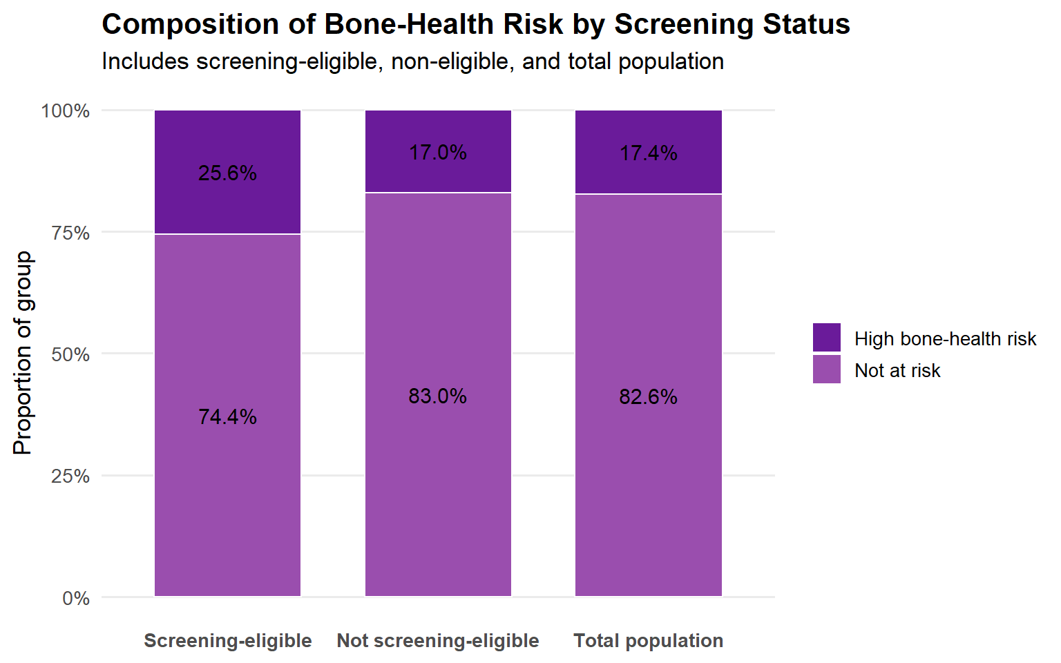
The below plot shows the proportion of individuals classified as high bone risk within each screening eligibility group (screening-eligible, not screening-eligible) as well as within the total population.
In particular, it highlights that a substantial portion of those who are not age-eligible for screening meet high-risk criteria. Of the 125 individuals who were screening eligible, 25.6% were also high bone risk. Of the sample that is not eligible for screening, 17% is at high bone-health risk. Similalry, 17.4% of the total sample is a high bone-health risk.
# Risk Composition by Screening Eligibility
plot1 <- data %>%
  mutate(
    screening_group = if_else(
      screening_eligible == 1,
      "Screening-eligible",
      "Not screening-eligible"
    ),
    risk_group = if_else(
      high_bone_risk == 1,
      "High bone-health risk",
      "Not at risk"
    )
  ) %>%
  # Create total population rows
  bind_rows(
    data %>%
      mutate(
        screening_group = "Total population",
        risk_group = if_else(
          high_bone_risk == 1,
          "High bone-health risk",
          "Not at risk"
        )
      )
  ) %>%
  count(screening_group, risk_group) %>%
  group_by(screening_group) %>%
  mutate(pct = n / sum(n)) %>%
  ungroup() %>%
  mutate(
    screening_group = factor(
      screening_group,
      levels = c(
        "Screening-eligible",
        "Not screening-eligible",
        "Total population"
      )
    )
  )


# Rendering plot
ggplot(plot1, aes(x = screening_group, y = pct, fill = risk_group)) +
  geom_col(width = 0.7, color = "white", linewidth = 0.5) +
  geom_text(
    aes(label = percent(pct, accuracy = 0.1)),
    position = position_stack(vjust = 0.5),
    size = 4
  ) +
  scale_y_continuous(labels = percent_format(accuracy = 1)) +
  scale_fill_manual(
    values = c(
      "High bone-health risk" = "#6A1B9A",  # deep purple
      "Not at risk" = "#9A4EAE"             # lighter purple
    )
  ) +
  labs(
    title = "Composition of Bone-Health Risk by Screening Status",
    subtitle = "Includes screening-eligible, non-eligible, and total population",
    x = NULL,
    y = "Proportion of group",
    fill = NULL
  ) +
  theme_minimal(base_size = 13) +
  theme(
    plot.title = element_text(face = "bold"),
    axis.text.x = element_text(face = "bold"),
    panel.grid.major.x = element_blank(),
    panel.grid.minor = element_blank()
  )
The table below presents age- and gender-specific segment sizes alongside corresponding rates of screening eligible, high bone risk and missed high risk. This view highlights how both the magnitude and concentration of missed bone-health risk vary across demographic groups under current screening criteria.
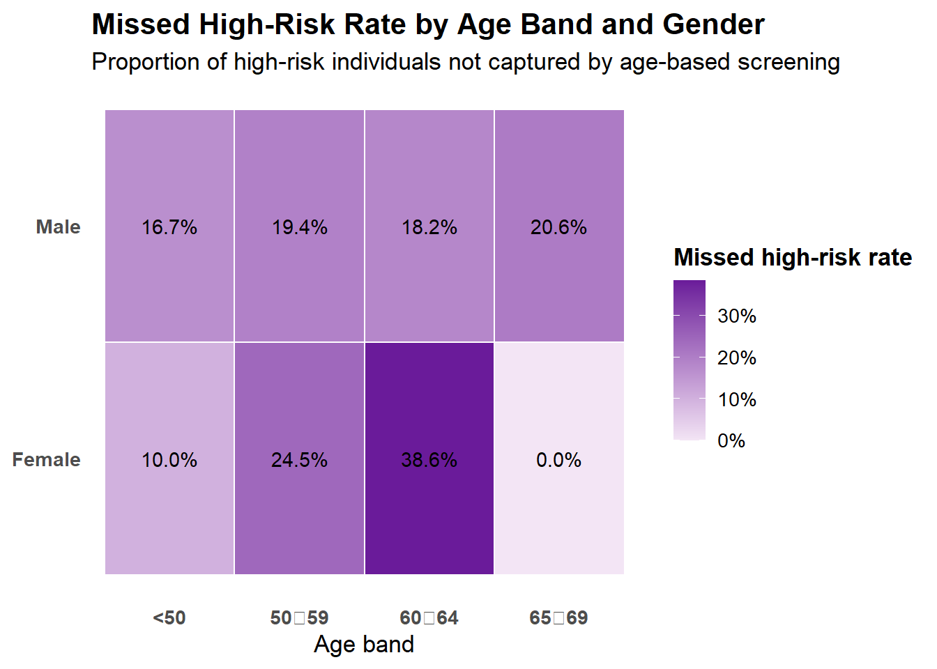
The table shows that all screening eligible individuals come from a single demographic group, females ages 65-69. It also highlights which demographic groups have large missed high risk rates (such as females aged 60-64 [38.6%], females aged 50-59 [24.5%]).
# Segment ranking (what population groups are most affect)

# Preparing demographic variables
data %<>%
  mutate(
    gender = factor(if_else(RIAGENDR == 2, "Female", "Male"),
                 levels = c("Female", "Male")),
age_band = cut(
      RIDAGEYR,
      breaks = c(0, 49, 59, 64, 69, 79, Inf),
      labels = c("<50", "50\u201159", "60\u201164", "65\u201169", "70\u201179", "80+"),
      right = TRUE
    ),
    age_band = factor(
      age_band,
      levels = c("<50", "50\u201159", "60\u201164", "65\u201169", "70\u201179", "80+"),
      ordered = TRUE
    )
  )

# Preparing data
segment_core <- data %>%
  group_by(age_band, gender) %>%
  summarise(
    n = n(),
    screening_eligible_n = sum(screening_eligible == 1, na.rm = TRUE),
    screening_eligible_rate = screening_eligible_n / n,
    high_risk_n = sum(high_bone_risk == 1, na.rm = TRUE),
    high_risk_rate = high_risk_n / n,
    missed_high_risk_n = sum(missed_high_risk == 1, na.rm = TRUE),
    missed_high_risk_rate = missed_high_risk_n / n,

    .groups = "drop"
  )

# Making table
kable(
  segment_core %>%
    mutate(
      screening_eligible_rate = percent(screening_eligible_rate, accuracy = 0.1),
      high_risk_rate = percent(high_risk_rate, accuracy = 0.1),
      missed_high_risk_rate = percent(missed_high_risk_rate, accuracy = 0.1)
    ),
  col.names = c(
    "Age Band",
    "Gender",
    "Population (N)",
    "Screening Eligible (N)",
    "Screening Eligible Rate",
    "High Bone Risk (N)",
    "High Bone Risk Rate",
    "Missed High Risk (N)",
    "Missed High Risk Rate"
  ),
   align = c("l", "l", "r", "r", "r", "r", "r", "r", "r"),
  caption = "Segment ranking by age band and gender using core cohort definitions"
)| Age Band | Gender | Population (N) | Screening Eligible (N) | Screening Eligible Rate | High Bone Risk (N) | High Bone Risk Rate | Missed High Risk (N) | Missed High Risk Rate |
|---|---|---|---|---|---|---|---|---|
| <50 | Female | 933 | 0 | 0.0% | 93 | 10.0% | 93 | 10.0% |
| <50 | Male | 1027 | 0 | 0.0% | 171 | 16.7% | 171 | 16.7% |
| 50‑59 | Female | 282 | 0 | 0.0% | 69 | 24.5% | 69 | 24.5% |
| 50‑59 | Male | 279 | 0 | 0.0% | 54 | 19.4% | 54 | 19.4% |
| 60‑64 | Female | 166 | 0 | 0.0% | 64 | 38.6% | 64 | 38.6% |
| 60‑64 | Male | 154 | 0 | 0.0% | 28 | 18.2% | 28 | 18.2% |
| 65‑69 | Female | 125 | 125 | 100.0% | 32 | 25.6% | 0 | 0.0% |
| 65‑69 | Male | 141 | 0 | 0.0% | 29 | 20.6% | 29 | 20.6% |
The heatmap below is a visual representation of this, highlighting age–gender segments with the greatest screening gaps, where a higher portion of high-risk individuals are not captured by current age-based screening criteria. Color intensity reflects the magnitude of missed high-risk prevalence within each segment.
# Missed High-Risk Heatmap
plot2 <- data %>%
  group_by(age_band, gender) %>%
  summarise(missed_rate = mean(missed_high_risk, na.rm = TRUE),
            n = n(),
            .groups = "drop")

# Rendering plot
ggplot(plot2, aes(x = age_band, y = gender, fill = missed_rate)) +
  geom_tile(color = "white", linewidth = 0.4) +
  geom_text(
    aes(label = percent(missed_rate, accuracy = 0.1)),
    size = 3.8,
    color = "black"
  ) +
  scale_fill_gradient(
    low = "#F3E5F5",   # very light purple
    high = "#6A1B9A",  # deep purple
    labels = percent_format(accuracy = 1)
  ) +
  labs(
    title = "Missed High-Risk Rate by Age Band and Gender",
    subtitle = "Proportion of high-risk individuals not captured by age-based screening",
    x = "Age band",
    y = NULL,
    fill = "Missed high-risk rate"
  ) +
  theme_minimal(base_size = 13) +
  theme(
    panel.grid = element_blank(),
    plot.title = element_text(face = "bold"),
    axis.text.x = element_text(face = "bold"),
    axis.text.y = element_text(face = "bold"),
    legend.title = element_text(face = "bold")
  )
The table below summarizes the prevalence of selected clinical and lifestyle risk factors related to bone health across the analytic population. Values represent the percentage of individuals exhibiting each risk factor and provide context for subsequent cohort and driver analyses.
In the total sample, reduced bone density was common, with 22% of individuals classified as having lumbar spine osteopenia and a further 2% meeting criteria for osteoporosis. Behavioral and clinical risk factors were also prevalent, including smoking (48%), low physical activity (33%), and prior fracture history (12%), underscoring the multifaceted nature of bone-health risk beyond age alone.
# Risk factor prevalence in the population
risk_summary <- data %>%
  summarise(
    low_bmi = mean(low_bmi == 1, na.rm = TRUE),
    osteopenia = mean(spine_class == 1, na.rm = TRUE),
    osteoporosis = mean(spine_class == 2, na.rm = TRUE),
    smoker = mean(smoker_status %in% c(1, 2), na.rm = TRUE),
    prior_fracture = mean(prior_fracture == 1, na.rm = TRUE),
    low_activity = mean(PAD200 == 2 & PAD320 == 2, na.rm = TRUE)
  ) %>%
  pivot_longer(everything(),
               names_to = "driver",
               values_to = "prevalence") %>%
  mutate(prevalence = round(prevalence, 2),
         prevalence = percent(prevalence)
  ) %>%
   mutate(
    driver = recode(
      driver,
      low_bmi        = "Low body mass index (BMI < 18.5)",
      osteopenia    = "Lumbar spine osteopenia (T-score −1.0 to −2.5)",
      osteoporosis  = "Lumbar spine osteoporosis (T-score ≤ −2.5)",
      smoker        = "Current or former smoker",
      prior_fracture= "Prior fracture (hip, wrist, or spine)",
      low_activity  = "Low physical activity"
    )
  )

kable(risk_summary, col.names = c("Driver", "Prevalence"), caption = "Risk Factor Prevalence in the Total Sample")| Driver | Prevalence |
|---|---|
| Low body mass index (BMI < 18.5) | 2% |
| Lumbar spine osteopenia (T-score −1.0 to −2.5) | 22% |
| Lumbar spine osteoporosis (T-score ≤ −2.5) | 2% |
| Current or former smoker | 48% |
| Prior fracture (hip, wrist, or spine) | 12% |
| Low physical activity | 33% |
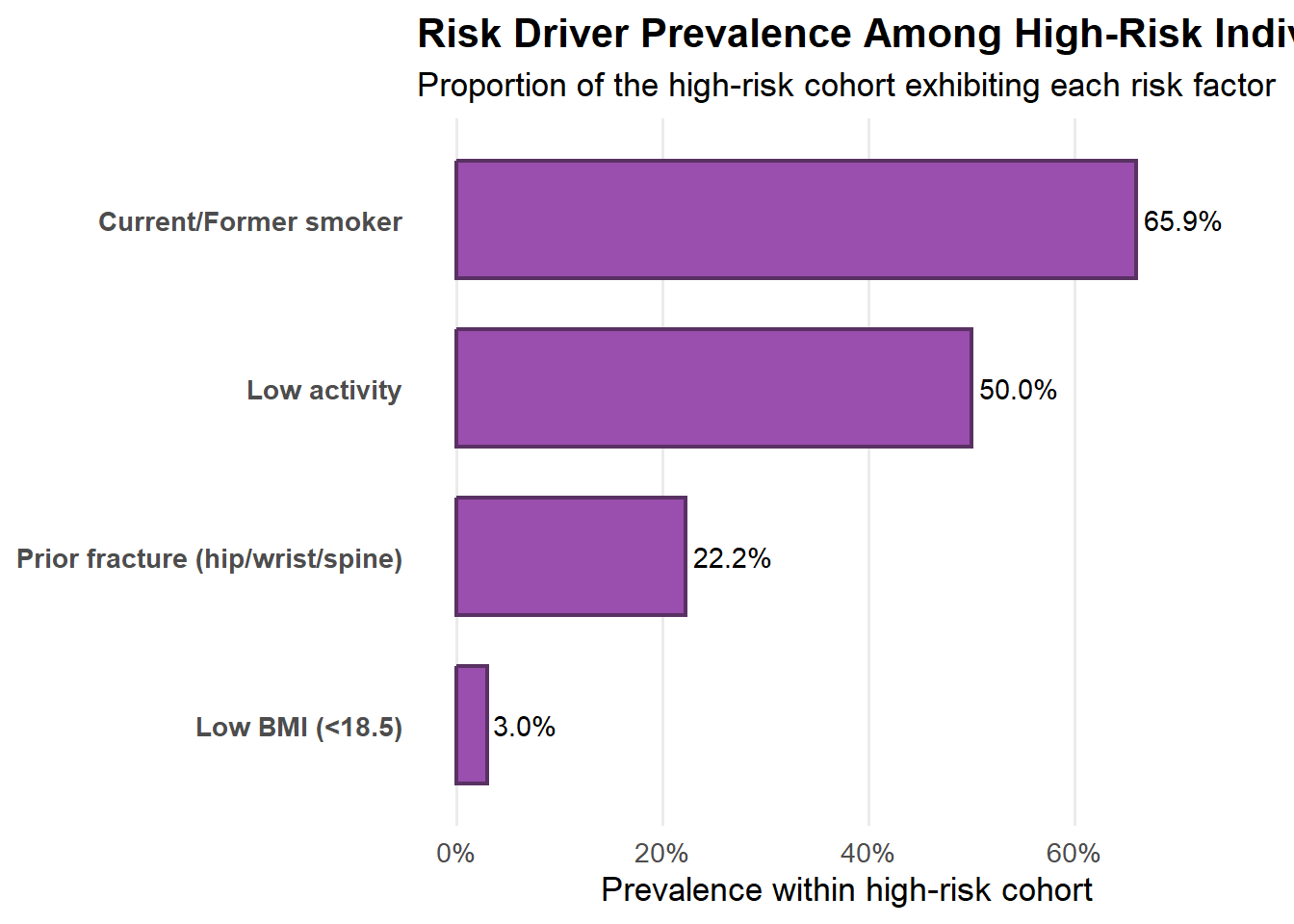
The table below summarizes the prevalence of selected clinical and lifestyle risk factors related to bone health across the high-risk sample. Values represent the percentage of individuals exhibiting each risk factor and provide context for subsequent cohort and driver analyses. Among individuals classified as high bone risk, reduced bone density was dominant, with 13% meeting criteria for lumbar spine osteoporosis and 87% exhibiting osteopenia. Lifestyle and clinical risk factors remained highly prevalent, particularly being a current or former smoker (66%), low physical activity (50%), prior fracture history (22%), and low body mass index (3%), highlighting multiple, overlapping contributors to elevated bone-health risk.
# Risk factor prevalence in the high risk sample
risk_summary <- data %>%
  filter(high_bone_risk == 1) %>%
  summarise(
    low_bmi = mean(low_bmi == 1, na.rm = TRUE),
    osteopenia = mean(spine_class == 1, na.rm = TRUE),
    osteoporosis = mean(spine_class == 2, na.rm = TRUE),
    smoker = mean(smoker_status %in% c(1, 2), na.rm = TRUE),
    prior_fracture = mean(prior_fracture == 1, na.rm = TRUE),
    low_activity = mean(PAD200 == 2 & PAD320 == 2, na.rm = TRUE)
  ) %>%
  pivot_longer(everything(),
               names_to = "driver",
               values_to = "prevalence") %>%
  mutate(prevalence = round(prevalence, 2),
         prevalence = percent(prevalence)
  ) %>%
   mutate(
    driver = recode(
      driver,
      low_bmi        = "Low body mass index (BMI < 18.5)",
      osteopenia    = "Lumbar spine osteopenia (T-score −1.0 to −2.5)",
      osteoporosis  = "Lumbar spine osteoporosis (T-score ≤ −2.5)",
      smoker        = "Current or former smoker",
      prior_fracture= "Prior fracture (hip, wrist, or spine)",
      low_activity  = "Low physical activity"
    )
  )

kable(risk_summary, col.names = c("Driver", "Prevalence"), caption = "Risk Factor Prevalence in the High-Risk Sample")| Driver | Prevalence |
|---|---|
| Low body mass index (BMI < 18.5) | 3% |
| Lumbar spine osteopenia (T-score −1.0 to −2.5) | 87% |
| Lumbar spine osteoporosis (T-score ≤ −2.5) | 13% |
| Current or former smoker | 66% |
| Prior fracture (hip, wrist, or spine) | 22% |
| Low physical activity | 50% |
The below plot summarizes the distribution of key risk factors within the high-bone-risk cohort, illustrating which characteristics are most prevalent among individuals at elevated fracture risk. The results provide context for understanding how risk accumulates beyond bone density alone. Osteopenia and osteoporosis are not shown in this figure because bone density categories were used to define the high-risk cohort; the chart focuses on additional clinical and lifestyle risk factors present within that group.
# Risk Factor Prevalence (High-Risk Sample) plot
plot3 <- data %>%
  filter(high_bone_risk == 1) %>%
  summarise(
    `Low BMI (<18.5)` = mean(low_bmi == 1, na.rm = TRUE),
    `Current/Former smoker` = mean(smoker_status %in% c(1, 2), na.rm = TRUE),
    `Prior fracture (hip/wrist/spine)` = mean(prior_fracture == 1, na.rm = TRUE),
    `Low activity` = mean(PAD200 == 2 & PAD320 == 2, na.rm = TRUE)
  ) %>%
  pivot_longer(everything(), names_to = "driver", values_to = "rate") %>%
  arrange(rate)

max_rate <- max(plot3$rate, na.rm = TRUE)

ggplot(plot3, aes(x = rate, y = reorder(driver, rate))) +
  geom_col(width = 0.7, fill = "#9A4EAE", color = "#593163", linewidth = 0.8) +
  geom_text(aes(label = percent(rate, accuracy = 0.1)),
            hjust = -0.1, size = 3.8) +
  scale_x_continuous(
    labels = percent_format(accuracy = 1),
    limits = c(0, ifelse(is.finite(max_rate), max_rate * 1.15, 1))
  ) +
  labs(
    title = "Risk Driver Prevalence Among High-Risk Individuals",
    subtitle = "Proportion of the high-risk cohort exhibiting each risk factor",
    x = "Prevalence within high-risk cohort",
    y = NULL
  ) +
  theme_minimal(base_size = 13) +
  theme(
    plot.title = element_text(face = "bold"),
    axis.text.y = element_text(face = "bold"),
    panel.grid.major.y = element_blank(),
    panel.grid.minor = element_blank()
  )
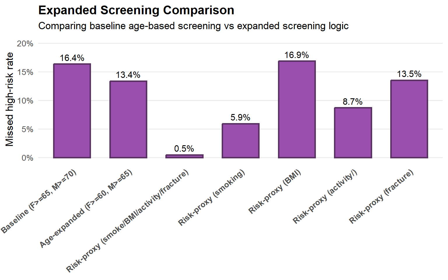
This below plot shows how different screening scenarios affect the proportion of high-risk individuals who would not be identified for screening. Individual-level screening eligibility was recalculated under each scenario, and the resulting missed high-risk rates were summarized at the population level to quantify the potential impact of expanding screening criteria.
Baseline: “What % of people are high risk and missed today (female >= 65, male >= 70)?”
Age-expanded: “What % would still be missed if we lowered age thresholds (female >= 60, male >= 65)?”
Risk-proxy: “What % would still be missed if we screened anyone with a risk proxy (smoker, low BMI, low activity, prior fracture)?”
Risk-proxy individual risks: “What % would still be missed if we screened anyone with one of the risk proxies (smoker, low BMI, low activity, prior fracture)?”
The below plot shows the proportion of the total population that is both high bone risk and not screening-eligible under the various scenarios.
Under current age-based screening criteria, approximately 16.4% of the total population is classified as high bone risk yet would not be identified for screening, indicating a substantial screening gap. Modest age-based expansion reduces this missed high-risk prevalence only marginally (to 13.4%), suggesting that age thresholds alone have limited impact. In contrast, screening triggered by simple risk proxies—such as smoking history, low BMI, low physical activity, or prior fracture—dramatically reduces the missed high-risk population to near zero, highlighting the potential value of risk-informed screening strategies over age-only approaches.
# Defining Scenarios
data %<>%
  mutate(
    # Baseline screening eligibility (original definition)
    screening_baseline = if_else(
      (RIAGENDR == 2 & RIDAGEYR >= 65) |
      (RIAGENDR == 1 & RIDAGEYR >= 70),
      1, 0
    ),

    # Age expanded scenario
    screening_age_expanded = if_else(
      (RIAGENDR == 2 & RIDAGEYR >= 60) |
      (RIAGENDR == 1 & RIDAGEYR >= 65),
      1, 0
    ),

    # Expanded risk proxies scenario (ANY of these triggers screening)
    screening_risk_proxy = if_else(
      (smoker_status %in% c(1, 2)) |
      (low_bmi == 1) |
      (low_activity == 1) |
      (prior_fracture == 1),
      1, 0
    ),

    # Expanded risk proxies scenario (smoking)
    screening_risk_proxy_smoking = if_else(
      (smoker_status %in% c(1, 2)),
      1, 0
    ),


    # Expanded risk proxies scenario (Low BMI)
    screening_risk_proxy_bmi = if_else(
      (low_bmi == 1),
      1, 0
    ),

    # Expanded risk proxies scenario (Low Activity)
    screening_risk_proxy_activity = if_else(
      (low_activity == 1),
      1, 0
    ),

    # Expanded risk proxies scenario (Prior Fracture)
    screening_risk_proxy_fracture = if_else(
      (prior_fracture == 1),
      1, 0
    ),

    # Missed high-risk under each definition (high risk but NOT eligible)
    missed_baseline = if_else(high_bone_risk == 1 & screening_baseline == 0, 1, 0),
    missed_age_expanded = if_else(high_bone_risk == 1 & screening_age_expanded == 0, 1, 0),
    missed_risk_proxy = if_else(high_bone_risk == 1 & screening_risk_proxy == 0, 1, 0),
    missed_risk_proxy_smoking = if_else(high_bone_risk == 1 & screening_risk_proxy_smoking == 0, 1, 0),
    missed_risk_proxy_lowBMI = if_else(high_bone_risk == 1 & screening_risk_proxy_bmi == 0, 1, 0),
    missed_risk_proxy_low_activity = if_else(high_bone_risk == 1 & screening_risk_proxy_activity == 0, 1, 0),
    missed_risk_proxy_prior_fracture = if_else(high_bone_risk == 1 & screening_risk_proxy_fracture == 0, 1, 0)
  )


# Measuring the impact of the scenarios - Proportion of the entire population that is both high bone risk and not screening-eligible under a given scenario.
plot4 <- tibble(
  scenario = c(
    "Baseline (F>=65, M>=70)",
    "Age-expanded (F>=60, M>=65)",
    "Risk-proxy (smoke/BMI/activity/fracture)",
    "Risk-proxy (smoking)",
    "Risk-proxy (BMI)",
    "Risk-proxy (activity/)",
    "Risk-proxy (fracture)"
  ),
  missed_rate = c(
    mean(data$missed_baseline, na.rm = TRUE),
    mean(data$missed_age_expanded, na.rm = TRUE),
    mean(data$missed_risk_proxy, na.rm = TRUE),
    mean(data$missed_risk_proxy_smoking, na.rm = TRUE),
    mean(data$missed_risk_proxy_lowBMI, na.rm = TRUE),
    mean(data$missed_risk_proxy_low_activity, na.rm = TRUE),
    mean(data$missed_risk_proxy_prior_fracture, na.rm = TRUE)
  )
) %>%
  mutate(
    scenario = factor(
      scenario,
      levels = c(
        "Baseline (F>=65, M>=70)",
        "Age-expanded (F>=60, M>=65)",
        "Risk-proxy (smoke/BMI/activity/fracture)",
        "Risk-proxy (smoking)",
        "Risk-proxy (BMI)",
        "Risk-proxy (activity/)",
        "Risk-proxy (fracture)"
      )
    )
  )


# Rendering the plot
ggplot(plot4, aes(x = scenario, y = missed_rate)) +
  geom_col(
    width = 0.65,
    fill = "#9A4EAE",     # light purple
    color = "#593163",    # dark purple outline
    linewidth = 0.9
  ) +
  geom_text(
    aes(label = percent(missed_rate, accuracy = 0.1)),
    vjust = -0.5,
    size = 4
  ) +
  scale_y_continuous(
    labels = percent_format(accuracy = 1),
    limits = c(0, max(plot4$missed_rate, na.rm = TRUE) * 1.2)
  ) +
  labs(
    title = "Expanded Screening Comparison",
    subtitle = "Comparing baseline age-based screening vs expanded screening logic",
    x = NULL,
    y = "Missed high-risk rate"
  ) +
  theme_minimal(base_size = 13)+
  theme(
    plot.title = element_text(face = "bold"),
    axis.text.x = element_text(
      face = "bold",
      angle = 40,     # rotate labels
      hjust = 1,      # right-align
      vjust = 1
    ),
    panel.grid.major.x = element_blank(),
    panel.grid.minor = element_blank()
  )
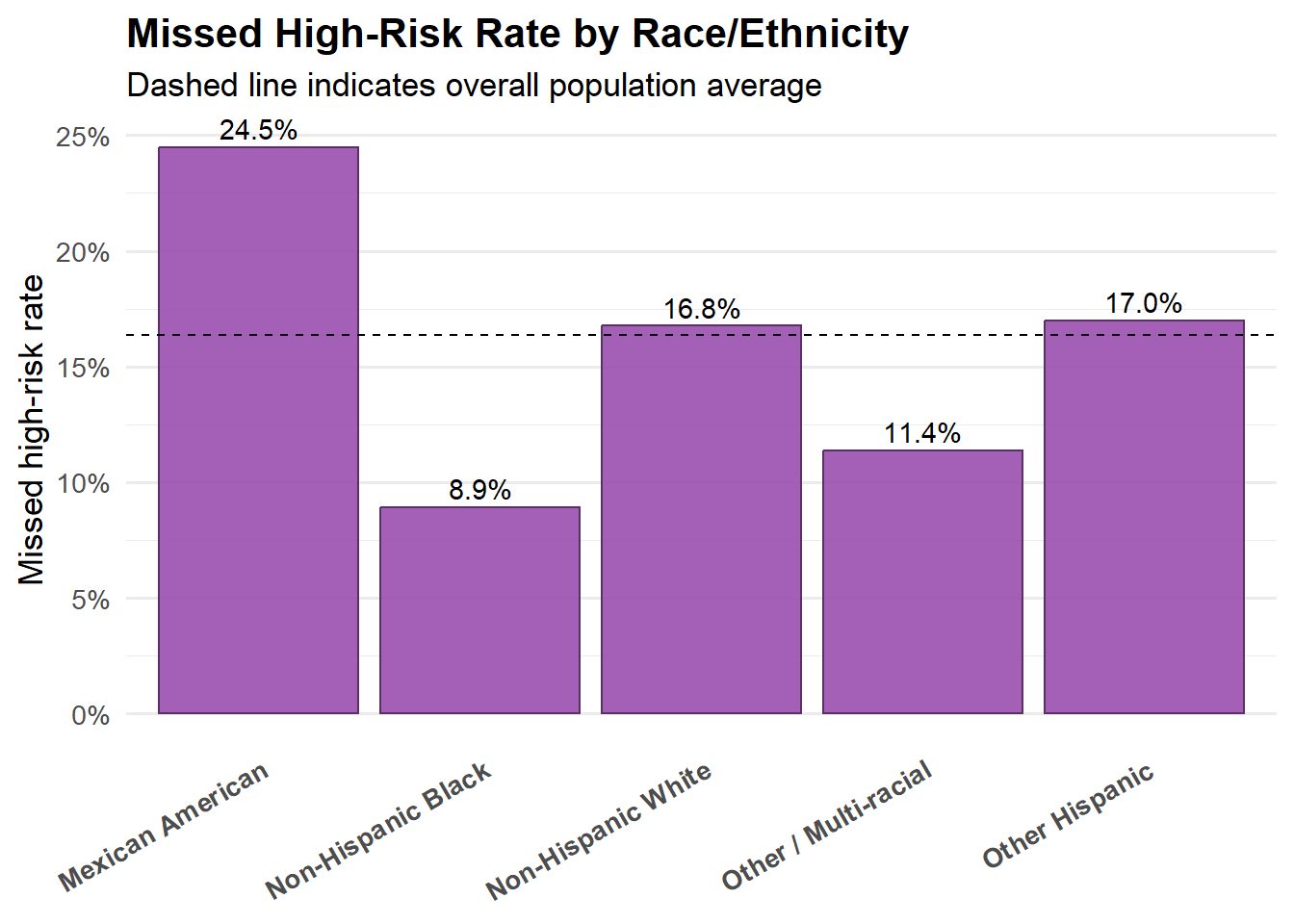
The below plot compares the population-level missed high-risk rate across racial groups, with the dashed line indicating the overall sample average. The figure is intended as an equity guardrail, highlighting whether missed high-risk prevalence differs meaningfully across groups rather than to support causal interpretation.
Missed high-risk prevalence varies across racial groups, with Mexican American sample showing higher-than-average missed rates, while Non-Hispanic Black and Other/Multi-racial individuals fall below the overall mean. Overall, the differences suggest that the screening gap is present across all groups, with some variation in magnitude rather than concentration in a single population.
# Racial Equity Plot
equity_bar <- data %>%
  group_by(race) %>%
  summarise(
    missed_rate = mean(missed_high_risk, na.rm = TRUE),
    n = n(),
    .groups = "drop"
  )

# Overall missed average
overall_missed <- mean(data$missed_high_risk, na.rm = TRUE)

# Rendering plot
ggplot(equity_bar, aes(x = race, y = missed_rate)) +
  geom_col(fill = "#9A4EAE",     # light purple
    color = "#593163",    # dark purple outline
    alpha = 0.9) +
  geom_hline(
    yintercept = overall_missed,
    linetype = "dashed",
    color = "black"
  ) +
  geom_text(
    aes(label = percent(missed_rate, accuracy = 0.1)),
    vjust = -0.4,
    size = 3.8
  ) +
  scale_y_continuous(labels = percent_format(accuracy = 1)) +
  labs(
    title = "Missed High-Risk Rate by Race/Ethnicity",
    subtitle = "Dashed line indicates overall population average",
    x = NULL,
    y = "Missed high-risk rate"
  ) +
  theme_minimal(base_size = 13) +
  theme(
    plot.title = element_text(face = "bold"),
    axis.text.x = element_text(
      face = "bold",
      angle = 30,     # rotate labels
      hjust = 1,      # right-align
      vjust = 1
    ),
    panel.grid.major.x = element_blank()

  )
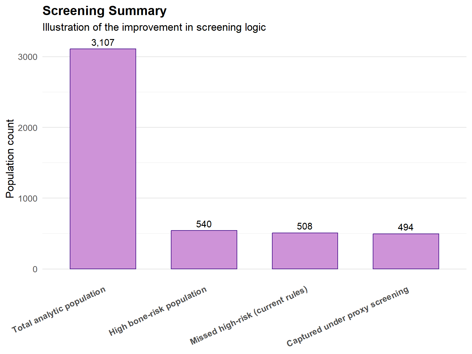
This analysis demonstrates that current age-based osteoporosis screening criteria are insufficient and capture only a small portion of individuals at elevated bone-health risk, leaving a substantial proportion of high-risk individuals unidentified. Risk is driven by a combination of structural bone deficits and common, readily observable factors such as low BMI, low physical activity, smoking history, and prior fracture history. Modest age-based expansion provides limited improvement, whereas incorporating simple risk proxies substantially reduces missed high-risk prevalence with minimal added complexity. These findings support a shift toward risk-informed screening strategies to improve identification efficiency and reduce preventable fracture risk.
# Summary plot
market_funnel <- tibble(
  stage = c(
    "Total analytic population",
    "High bone-risk population",
    "Missed high-risk (current rules)",
    "Captured under proxy screening"
  ),
  count = c(
    nrow(data),
    sum(data$high_bone_risk == 1, na.rm = TRUE),
    sum(data$missed_baseline == 1, na.rm = TRUE),
    sum(data$missed_baseline == 1, na.rm = TRUE) -
      sum(data$missed_risk_proxy == 1, na.rm = TRUE)
  )
)

ggplot(market_funnel,
       aes(x = reorder(stage, -count), y = count)) +
  geom_col(
    fill = "#CE93D8",
    color = "#4A148C",
    width = 0.65
  ) +
  geom_text(aes(label = scales::comma(count)),
            vjust = -0.5,
            size = 4) +
  labs(
    title = "Screening Summary",
    subtitle = "Illustration of the improvement in screening logic",
    x = NULL,
    y = "Population count"
  ) +
  theme_minimal(base_size = 13) +
  theme(
    plot.title = element_text(face = "bold"),
    axis.text.x = element_text(face = "bold", angle = 25, hjust = 1),
    panel.grid.major.x = element_blank()
  )
# Scaled based on Exam weight, PSU and stratum
# 1. Define survey design
nhanes_design <- svydesign(
  id = ~SDMVPSU,
  strata = ~SDMVSTRA,
  weights = ~WTMEC2YR,
  data = data,
  nest = TRUE
)

# 2. Calculate weighted proportion
weighted_result <- svymean(~missed_high_risk, nhanes_design)

weighted_result
mean SE
missed_high_risk 0.15215 0.0104confint(weighted_result) 2.5 % 97.5 %
missed_high_risk 0.1317964 0.1725016Using survey-weighted 2005–2006 data from the National Health and Nutrition Examination Survey, 15.22% of U.S. adults aged ≥20 met the expanded high-risk definition for poor bone health after properly accounting for the complex survey design (exam weights, strata, and clustering). Assuming a current U.S. adult (≥20) population of approximately 250 million, and assuming stable prevalence over time, this translates to an estimated:
250,000,000 × 0.1522 = 38,050,000
≈ 38.1 million U.S. adults who may represent an under-identified high-risk population under expanded screening criteria.
Xue, S., Zhang, Y., Qiao, W., Zhao, Q., Guo, D., Li, B., Shen, X., Feng, L., Huang, F., Wang, N., Oumer, K. S., Getachew, C. T., & Yang, S. (2021). An Updated Reference for Calculating Bone Mineral Density T-Scores. The Journal of Clinical Endocrinology and Metabolism, 106(7), e2613–e2621. https://doi.org/10.1210/clinem/dgab180